semiIVreg: R package for semi-IV regression

Christophe Bruneel-Zupanc

last modified: 2025-01-31

Overview

This package provides estimation procedure with semi-IVs, as in Bruneel-Zupanc (2024).
In particular, the main function semiivreg() estimates the marginal treatment effect (MTE) and marginal treatment response (MTR).

Installation

The development version of semiIVreg is hosted on GitHub here. It can be conveniently installed via the install_github() function from the remotes package.

remotes::install_github("cbruneelzupanc/semiIVreg")

semi-instrumental variable (semi-IV) regression

The model

semiivreg estimates the marginal treatment effect (MTE) and marginal treatment response (MTR) of the following model.

The potential outcomes are given by the semi-parametric model:

$$Y_0 = \delta_{0} + W_0 \beta_0 + X \beta^X_{0} + U_0, \quad \quad \quad (1)$$

$$Y_1 = \delta_{1} + W_1 \beta_1 + X \beta^X_{1} + U_1, \quad \quad \quad (2)$$

with selection rule

$$\begin{aligned} D^* &= g(W_0, W_1, X) - V \\ &= (\alpha + \alpha_0 W_0 + \alpha_1 W_1 + \alpha_{X} X ) - V, \quad \quad \quad (3) \\ \text{ with } \quad D &= \mathbb{I}(D^* > 0), \end{aligned}$$

where

• semi-IVs: $W_0$ (respectively $W_1$) are the semi-IVs excluded from $Y_1$ (resp. $Y_0$). Each $W_0$ and $W_1$ may contain several variables. Nonparametric identification requires that each $W_d$ contains at least one excluded variable (see Bruneel-Zupanc (2024)).

• Covariates: $X$ are the covariates that affect both potential outcomes. By default, different effect of the covariates across alternatives, (i.e., $\beta^X_{0} \neq \beta^X_{1}$). To do so, include the covariates separately in both MTR formulas: semiivreg(y~d|w0+x|w1+x, data). One can restrict the effect of $X$ to be the same across both potential outcomes (i.e., $\beta^X_{0} = \beta^X_{1}$). To do so, specify: semiivreg(y~d|w0|w1|x, data).

• Unobservables: $U_0$ and $U_1$ are general unobservables (may include several shocks, some may be the same across alternatives) affecting the outcomes. Generally normalize $E(U_d | X, W_d)=0$. $V$ is a scalar unobservable that affects the selection. The lower $V$, the more likely one is to select into treatment. Nonparametric identification requires independence, i.e., $(U_0, U_1, V) \perp (W_0, W_1) | X$.
  For estimation here, we additionally assume additive separability of the covariates $X$, i.e., that $E(U_d | V, X) = E(U_d | V)$ for both $d=0,1$.
  This assumption is not necessary for the identification, nor for the estimation. But it is a standard simplification that helps the estimation. See Carneiro, Heckman, and Vytlacil (2011), Brinch, Mogstad, and Wiswall (2017) or Andresen (2018) for comparable examples of the estimation of MTE with IVs.

Remark about the flexibility of the model: note that $W_0$ and $W_1$ can be flexible transformations (polynomial, splines) of specific variables, so the outcome equations are quite flexible (could also specify interactions between $W_d$ and $X$). The semi-parametric model main assumption here is the separability between the unobservables and $X, W_d$, otherwise the model is as general as it can be.

Estimation procedure

The estimation procedure closely follows the counterpart estimation of MTE with standard IVs, see for e.g., Andresen (2018). The command estimates Marginal Treatment Responses (MTR) and Marginal Treatment Effects (MTE). Define the normalized unobserved resistance to treatment $U_D = F_V(V) \sim Uniform(0, 1)$. Then, the MTRs are given by: $$\begin{aligned} MTR_d(u, w_d, x) &= E(Y_d | X=x, W_d=w_d, U_D=u) \\ &= \delta_{d} + W_d \beta_d + X \beta^X_{d} + E(U_d|X=x, W_d=w_d, U_D=u) \\ &= \delta_{d} + W_d \beta_d + X \beta^X_{d} + E(U_d|U_D=u) \\ &= \delta_{d} + W_d \beta_d + X \beta^X_{d} + k_d(u), \end{aligned}$$ where the last equalities comes from the fact that $E(U_d|X=x, W_d=w_d, U_D=u) = E(U_d|U_D=u)$ by the separability and independence, and then we just define $k_d(u) = E(U_d|U_D=u)$.

Then, the Marginal Treatment Effects (MTE) are given by $$\begin{aligned} MTE(u, x, w_0, w_1) &= E(Y_1 - Y_0 | X = x, W_0=w_0, W_1=w_1, U_D=u) \\ &= MTR_1(u, w_1, x) - MTR_0(u, w_0, x). \end{aligned}$$

Remark: the MTR and MTE are estimated at given covariates and semi-IVs, $(X, W_0, W_1)$. This is specified using ref_indiv. Or by default, it computes the ‘average individual’ (and take reference level for factor).

The estimation proceeds in two stages: first estimate the propensity to be treated, $P$, and then the potential outcome treatment parameters.

1st stage: propensity score

Estimate the propensity score $\widehat{P}$ of treatment selection of equation (3).
By default, the function $g(\cdot)$ is given by the simple linear specification above, but the code allows specifying any other first stage. For example:

  semiivreg(y~d|w0+x|w1+x, data,
            propensity_formula = d~w0+w1+w0:w1+w0:x+w1:x+I(w0^2)+I(w1^2))

By default, the estimation assumes a probit model for the first stage (i.e., assumes $V$ is normally distributed). However, you can specify other models (e.g., logit) using the firststage_model argument. In theory, any specification for the first stage could be added, and it is even possible to estimate the propensity score outside of the semiivreg command (this feature is not implemented yet).

2nd stage: marginal treatment responses

Estimated objects

First, given estimated $\widehat{P}$, the second stage estimates the following semi-parametric partially linear model for the potential outcomes $$\begin{aligned} E[Y|D=0, W_0, X, \widehat{P}] &= \delta_{0} + W_0 \beta_0 + X \beta^X_{0} + \kappa_0(\widehat{P}), \\ E[Y|D=1, W_1, X, \widehat{P}] &= \delta_{1} + W_1 \beta_1 + X \beta^X_{1} + \kappa_1(\widehat{P}), \end{aligned}$$ where $\kappa_d(P)$ are control functions, equal to $$\begin{aligned} \kappa_1(P) &= E[ U_1 | D=1, W_1, W_0, X,P] = E[U_1|D=1, P] = E[U_1 | U_D \leq P] \\ \kappa_0(P) &= E[ U_0 | D=0, W_1, W_0, X,P] = E[U_0|D=0, P] = E[U_0 | U_D > P]. \end{aligned}$$ It is a partially linear model because the control functions are nonparametric and can be estimated more or less flexibly (see below).

Once the parameters $\delta_d, \beta_d, \beta^X_d$ and the flexible control function $\kappa_d()$ are estimated, we don’t need to estimate any other parameters to obtain the MTE and MTR. We only need to also obtain the derivative from the estimated $\kappa_d$. Indeed, define $$\begin{aligned} \widehat{k}_1(u) &= E[ U_1 | U_D=u] = \widehat{\kappa}_1(u) + u \widehat{\kappa}_1'(u), \\ \widehat{k}_0(u) &= E[ U_0 | U_D=u] = \widehat{\kappa}_0(u) - (1-u) \widehat{\kappa}_0'(u). \end{aligned}$$

Then, the Marginal Treatment Responses are given by: $$\begin{aligned} \widehat{MTR}_d(u, w_d, x) &= E(Y_d | X=x, W_d=w_d, U_D=u) = \widehat{\delta}_{d} + w_d \widehat{\beta}_d + x \widehat{\beta}^X_{d} + \widehat{k}_d(u) \end{aligned}$$

and the Marginal Treatment Effects are: $$\begin{aligned} \widehat{MTE}(u, x, w_0, w_1) = \widehat{MTR}_1(u, w_1, x) - \widehat{MTR}_0(u, w_0, x). \end{aligned}$$

Consequently, the estimation is about estimating the parameters and $\kappa_d$. Several estimation method est_method are implemented in semiivreg(). We describe them below.

Method 1. Double residual regression, Robinson (1988)

The default method, implemented with est_method="locpoly" is to run a double residual regression, à la Robinson (1988), in order to estimate the partially linear model. We implement it similarly to the separate approach of Andresen (2018) for the estimation of MTE with IVs. We estimate using a separate approach, i.e., estimate separately on the treated and untreated samples, by implementing the following steps:

• Step 1. Estimate $E(Y_d | D=d, \widehat{P})$, $E(W_d | D=d, \widehat{P})$ and $E(X | D=d, \widehat{P})$ with a nonparametric local polynomial regression. To specify the bandwidth of the local polynomial regression, use bw0 or bw1. If not specified, the bandwidth are automatically computed using the method of bw_method. The default being a fast "1/5 rule, picking a bandwidth equal to 1/5th of the common support. We can also specify the degree of the polynomial with pol_degree_locpoly1. By default, equal to $1$ as recommended in Fan and Gijbels (1996) (order of the function we target $+1$).

• Step 2. On each subsample, compute the residuals $e_{Y_d} = Y_d - E(Y_d | D=d, \widehat{P})$, $e_{W_d} = W_d - E(W_d | D=d, \widehat{P})$ and $e_X^d = X - E(X | D=d, \widehat{P})$. Then, run the first residual regression, with a no-intercept OLS:
  $$e_{Y_d} = e_{W_d} \beta_d + e_X^d \beta^X_d + \tilde{U}_d.$$
  This regression on the subsample with $D=d$, provides consistent estimates of $\beta_d$ and $\beta^X_d$.
  Indeed, the residual equation is equivalent to
  $$Y_d - E[Y_d | D=d, \widehat{P}] = (W_d - E[W_d | D=d, \widehat{P}]) \beta_d + E(X - E[X | D=d, \widehat{P}]) \beta_d^X + (U_d - E[U_d | D=d, \widehat{P}]).$$ and if we denote $\tilde{U}_d = U_d - E[U_d | D=d, \widehat{P}]$, we have $E[\tilde{U}_d | D=d, \widehat{P}] = 0$, so the no-intercept residual OLS regression gives consistent estimates.

• Step 3. Construct $\tilde{Y}_d = Y - W_d \widehat{\beta_d} - X \widehat{\beta^X_d}$, on the sample with $D=d$, i.e., the outcome net of the effect of the covariates. We have $$\tilde{Y}_d = \delta_d + U_d.$$ This yields $$\tilde{\kappa}_d(P) = E[\tilde{Y}_d | D=d, P]$$

• Step 4. Estimate $\tilde{\kappa}_d(P)$ using a second nonparametric local polynomial regression of $\tilde{Y}_d$ on $P$. To specify the bandwidth of the local polynomial regression, use bw_y0 or bw_y1. If not specified, the bandwidth are automatically computed using the method of bw_method. The default is again the arbitrary 1/5th rule, but we recommend using "mse-dpi" for the direct plug-in MSE optimal bandwidth from Fan and Gijbels (1996), as implemented by in the nprobust package (Calonico, Cattaneo, and Farrell (2019)) instead. We can also specify the degree of the polynomial with pol_degree_locpoly2. By default, equal to $2$ as recommended in Fan and Gijbels (1996) because we want to estimate the derivative, $\tilde{k}_d(u) = E[\delta_d + U_d|U_D=u]$. Once we have $\tilde{\kappa}_d$, we can compute $$\begin{aligned} \widehat{\tilde{k}}_1(u) &= E[ \delta_1 + U_1 | U_D=u] = \widehat{\tilde{\kappa}}_1(u) + u \widehat{\tilde{\kappa}}_1'(u), \\ \widehat{\tilde{k}}_0(u) &= E[ \delta_0 + U_0 | U_D=u] = \widehat{\tilde{\kappa}}_0(u) - (1-u) \widehat{\tilde{\kappa}}_0'(u). \end{aligned}$$

Using the $\widehat{\tilde{k}}_d(u)$ and the estimated $\widehat{\beta}_d, \widehat{\beta}^X_d$, we can compute the MTR on this subsample $D=d$, as $$\begin{aligned} \widehat{MTR}_d(u, w_d, x) &= E(Y_d | X=x, W_d=w_d, U_D=u) = w_d \widehat{\beta}_d + x \widehat{\beta}^X_{d} + \widehat{\tilde{k}}_d(u). \end{aligned}$$
Remark that the definition of $\tilde{\kappa}_d(P)$, is equivalent to defining a more general shock that would include a constant, $\tilde{U}_d = \delta_d + U_d$. This is innoccuous and yield the same MTR/MTE in the end.

Once the MTR are estimated separately on both subsample, we can estimate the MTE: $$\begin{aligned} \widehat{MTR}_d(u, w_d, x) &= E(Y_d | X=x, W_d=w_d, U_D=u) = w_d \widehat{\beta}_d + x \widehat{\beta}^X_{d} + \widehat{\tilde{k}}_d(u) \\ \widehat{MTE}(u, x, w_0, w_1) &= \widehat{MTR}_1(u, w_1, x) - \widehat{MTR}_0(u, w_0, x). \end{aligned}$$

Advantages. The main advantage of this double residual regression is that it is robust to misspecification of the nonparametric $\kappa_d$ function, see Robinson (1988). However, it still requires to specify the bandwidths. In order to obtain the standard errors around the estimates, given that $P$ is estimated in a first stage, we bootstrap the standard errors using semiivreg_boot(). This function takes longer than the default estimation which is almost instantaneous.

Method 2. Sieve estimation

An alternative method is to use sieve approach, implemented with est_method="sieve", to estimate the second stage. The idea is simply to specify the control function $\kappa_d$ as a flexible function of $P$, using flexible functional form.

By default we use polynomial transformation of degree pol_degree_sieve=5 for $\kappa_0(P)$ and $\kappa_1(P)$. Then, we estimate the second stage using a stacked regression of the form: $$\begin{aligned} E[Y|W_0, W_1, X, \widehat{P}] = &D \times ( \delta_{1} + W_1 \beta_1 + X \beta^X_{1} + \kappa_1(\widehat{P}) ) + \\ &(1-D) \times ( \delta_{0} + W_0 \beta_0 + X \beta^X_{0} + \kappa_0(\widehat{P})). \end{aligned}$$ We do it as a stacked regression and not separately in order to allow to restrict some covariates to have the same effect on both potential outcomes (e.g., $\beta_0^X = \beta_1^X$).

Once we obtain $\widehat{\kappa}_d(P)$, we proceed as before to obtain $k_d(u)$ and the MTR/MTE. Because of the polynomial functional form, $k_d(u)$ has a known functional form based on the estimated coefficients for $\kappa_d$, so it is very easy to compute.

Advantages. The main advantage of this sieve approach is that it is faster and easier to implement (but "locpoly" is also fast anyway). It also provides analytical standard errors. These are wrong because they do not take into account that $\widehat{P}$ is estimated in a first stage, but, if $\widehat{P}$ is well estimated, the analytical standard errors should be very close to the true one that we can obtain with the bootstrap in semiivreg_boot().
The disadvantage is that it is less robust to misspecification of the control function as a polynomial. Even though, as visible in this vignette, it still works well in our examples, even if the underlying $\kappa_d$ is not a polynomial.

Method 3. Special Case with Homogenous Treatment Effects

Using est_method="homogenous", semiivreg() can also estimate a restricted model where we assume that the treatment effects are homogenous, i.e., the $MTE(u, x, w_0, w_1) = MTE(x, w_0, w_1)$, only varies with the observable covariates, but is constant with respect to $U_D$. The homogenous treatment effect assumption is equivalent to imposing that the underlying model corresponds to the general potential outcome model (1)-(2), with the additional restriction that $U_0 = U_1 = U$.

It is estimated using a procedure similar to the sieve approach with heterogenous treatment effects, but where we impose additional known restriction on the control functions $\kappa_0(P)$ and $\kappa_1(P)$ in the second stage estimation. Indeed, $$E(U) = 0 = E(U | U_D \leq P) P + E(U | U_D > P) (1-P)$$

So, $\kappa_0(P) = -\kappa_1(P) \frac{P}{1-P}$, and one can check that it yields $k_0(u) = k_1(u) = k(u)$.

Thus, the MTE is constant ($k_1(u) - k_0(u) = 0$, it cancels out), and equal to:

$$\widehat{MTE}(x, w_0, w_1) = \widehat{\delta}_{1} - \widehat{\delta}_{0} + w_1 \widehat{\beta}_1 - w_0 \widehat{\beta}_0 + x (\widehat{\beta}^X_{1} - \widehat{\beta}^X_{0}).$$

Note that the MTR still varies with $u$ because $k(u)$ is not constant, only the MTE is.

Caution about the Estimated Standard Errors

By default, est_method="sieve" and "homogenous” return analytic standard errors… But not accounting for the fact that the propensity score is estimated in a first stage in semiivreg. Thus, these are wrong (but the bias is very small if the first stage is well estimated, see these simulations for example).
Use semiivreg_boot to obtain ‘correct’ bootstrapped confidence intervals.

Illustration with simulated Roy model

This illustrates what the semiivreg()command reports for a semi-IV regression. By default, it reports the common support plot of the propensity score and the estimated marginal treatment effects (MTE). By default, the est_method = "locpoly" for Robinson (1988) double residual regression using local polynomial regressions.

library(semiIVreg)
data(roydata) # load the data from a simulated Roy model

# semi-IV regression
semiiv = semiivreg(y~d|w0|w1, data=roydata) 
#> Caution: the standard errors around the plot are not correct (underestimated) because of the multiple stages. For proper standard errors, run the bootstrap in semiivreg_boot().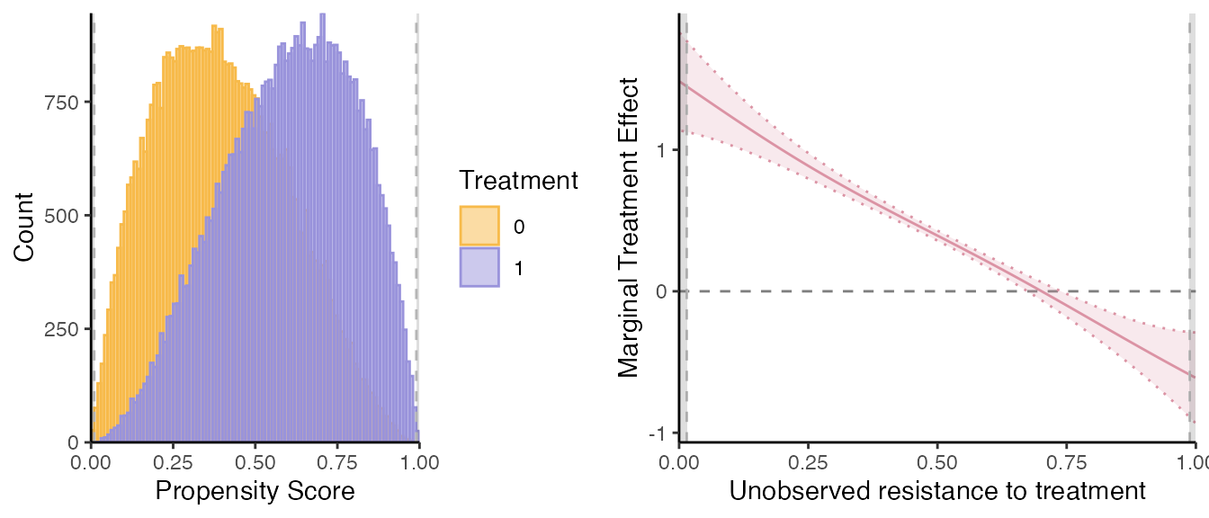

One can also easily extract a plot for the marginal treatment responses (MTR):

semiiv$plot$mtr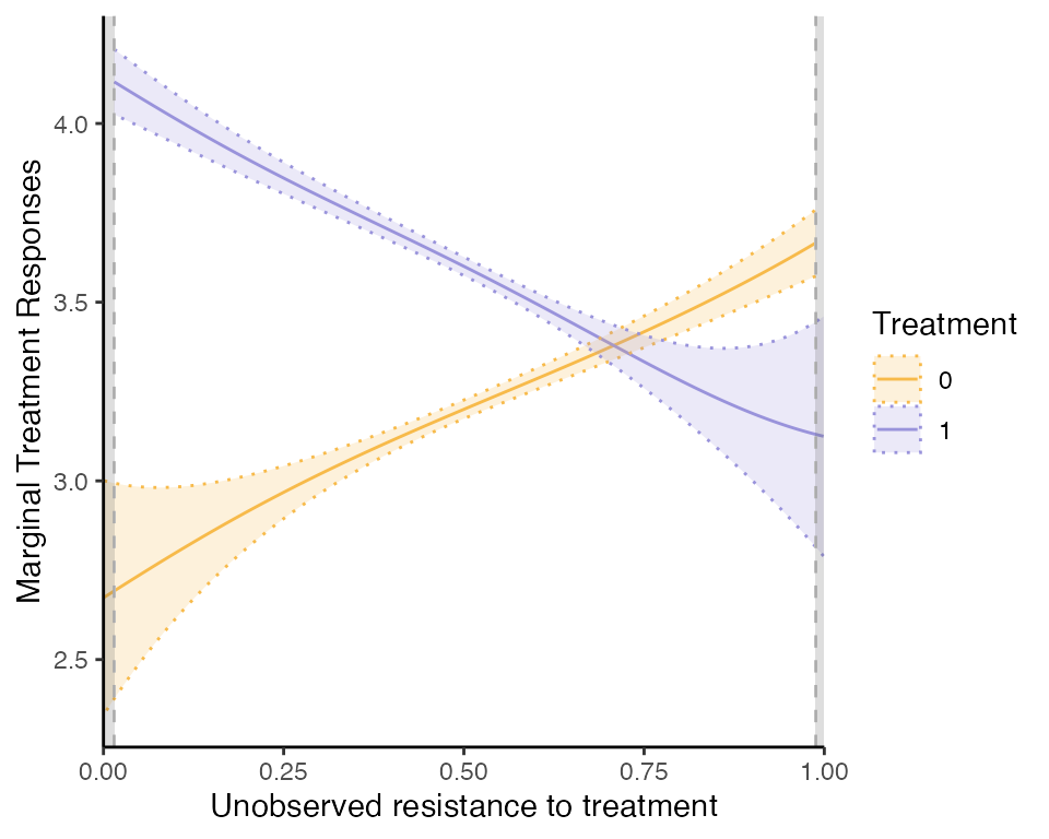

If one wants to use the sieve estimation method, simply run:

# semi-IV sieve regression
semiiv = semiivreg(y~d|w0|w1, data=roydata, est_method="sieve")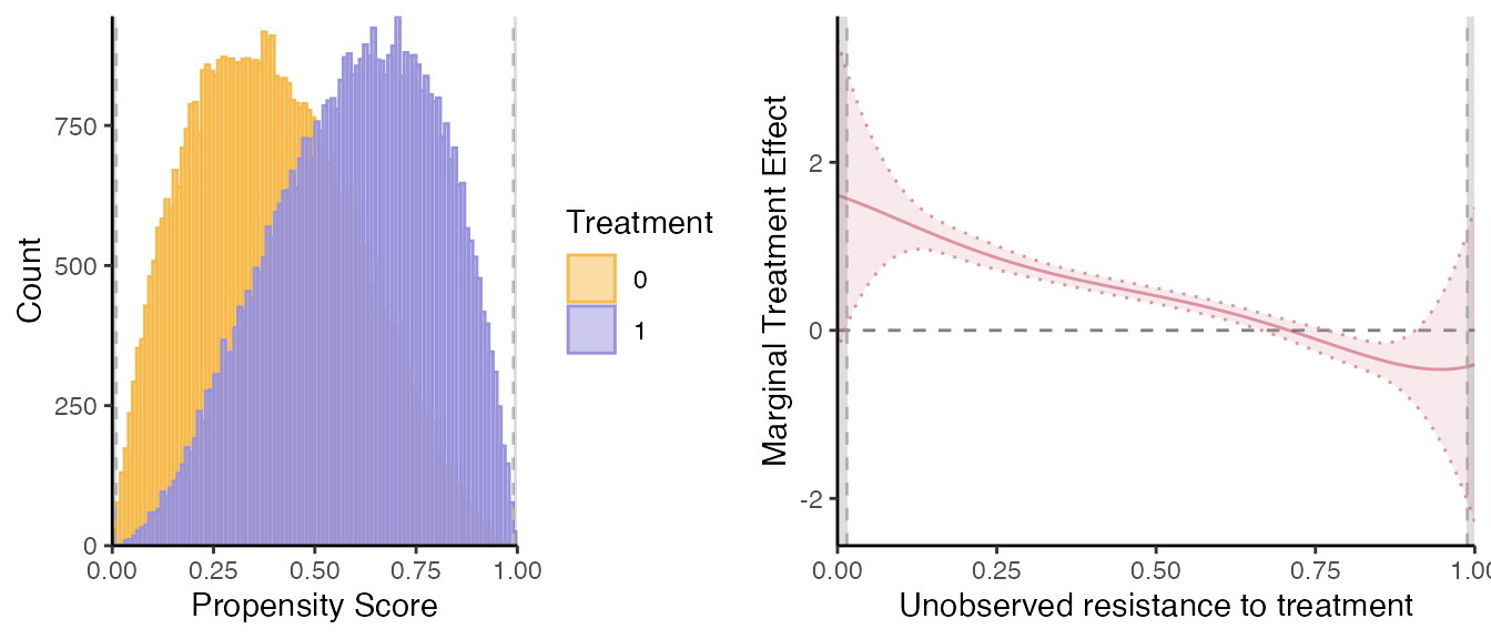 

semiiv$plot$mtr

One advantage of the sieve is that it reports confidence interval (though wrong because do not take into account the first stage error) and also gives a functional form for the MTR and MTE, obtainable by running the code below.

semiiv$est$mtr0; 
#>      Variable    Estimate    Std_Error      t_value     p_value
#> 1 (Intercept)   2.7581424 9.298226e-01   2.96631018 0.003014676
#> 2  kd(v): v^1  -0.6853761 1.229132e+01  -0.05576099 0.955532327
#> 3  kd(v): v^2  12.0175370 5.692871e+01   0.21109801 0.832811220
#> 4  kd(v): v^3 -30.6762292 1.188494e+02  -0.25811010 0.796322466
#> 5  kd(v): v^4  31.3667340 1.142864e+02   0.27445721 0.783733849
#> 6  kd(v): v^5 -10.8461651 4.113650e+01  -0.26366279 0.792040318
#> 7          w0   0.8002338 3.955818e-03 202.29288041 0.000000000
semiiv$est$mtr1; 
#>      Variable    Estimate    Std_Error      t_value       p_value
#> 1 (Intercept)   4.3655568  0.142511442  30.63302633 3.985092e-205
#> 2  kd(v): v^1  -3.2471062  3.735243561  -0.86931580  3.846765e-01
#> 3  kd(v): v^2   4.2847118 26.418324185   0.16218711  8.711588e-01
#> 4  kd(v): v^3   4.5087919 75.498769743   0.05972007  9.523787e-01
#> 5  kd(v): v^4 -17.9382899 93.543557546  -0.19176403  8.479274e-01
#> 6  kd(v): v^5  11.5530308 41.752329058   0.27670387  7.820081e-01
#> 7          w1   0.4977251  0.003904244 127.48309330  0.000000e+00
semiiv$est$mte
#>      Variable    Estimate    Std_Error      t_value    p_value
#> 1 (Intercept)   1.6074144 9.406804e-01    1.7087784 0.08749511
#> 2  kd(v): v^1  -2.5617302 1.284634e+01   -0.1994132 0.84193997
#> 3  kd(v): v^2  -7.7328252 6.275990e+01   -0.1232128 0.90193882
#> 4  kd(v): v^3  35.1850210 1.408021e+02    0.2498898 0.80267307
#> 5  kd(v): v^4 -49.3050239 1.476881e+02   -0.3338455 0.73849682
#> 6  kd(v): v^5  22.3991960 5.861287e+01    0.3821549 0.70234729
#> 7    + W1: w1   0.4977251 3.904244e-03  127.4830933 0.00000000
#> 8    - W0: w0  -0.8002338 3.955818e-03 -202.2928804 0.00000000

Similarly, homogenous treatment effects will also provide a functional form estimation.

For more details, see the vignettes on estimation with heterogenous or homogenous treatment effects. Refer also to Bruneel-Zupanc (2024).

References

Andresen, Martin Eckhoff. 2018. “Exploring Marginal Treatment Effects: Flexible Estimation Using Stata.” The Stata Journal 18 (1): 118–58.

Brinch, Christian N, Magne Mogstad, and Matthew Wiswall. 2017. “Beyond LATE with a Discrete Instrument.” Journal of Political Economy 125 (4): 985–1039.

Bruneel-Zupanc, Christophe. 2024. “Don’t (Fully) Exclude Me, It’s Not Necessary! Identification with Semi-IVs.” https://arxiv.org/abs/2303.12667.

Calonico, Sebastian, Matias D. Cattaneo, and Max H. Farrell. 2019. “Nprobust: Nonparametric Kernel-Based Estimation and Robust Bias-Corrected Inference.” Journal of Statistical Software 91 (8): 1–33. https://doi.org/10.18637/jss.v091.i08.

Carneiro, Pedro, James J. Heckman, and Edward J. Vytlacil. 2011. “Estimating Marginal Returns to Education.” The American Economic Review 101 (6): 2754–81. http://www.jstor.org/stable/23045657.

Fan, Jianqing., and Irène. Gijbels. 1996. Local Polynomial Modelling and Its Applications. Monographs on Statistics and Applied Probability 66. Boca Raton: Chapman; Hall/CRC.

Robinson, Peter M. 1988. “Root-n-Consistent Semiparametric Regression.” Econometrica: Journal of the Econometric Society, 931–54.